Quick start
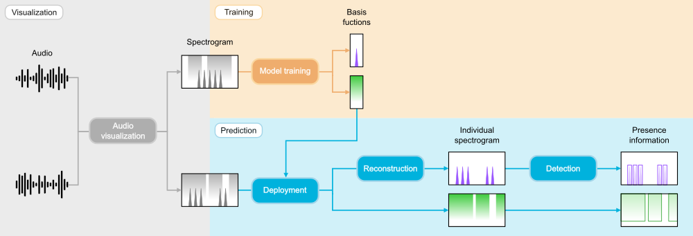
Visualizing audio data
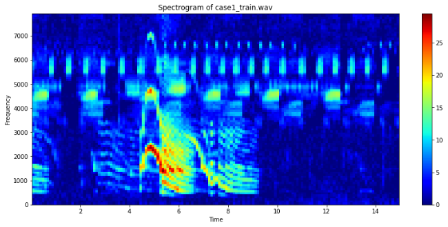
soundscape_IR provides a function audio_visualization to transform an audio into a spectrogram on the hertz or mel scale. It also enables the use of Welch’s averaging method and spectrogram prewhitening in noise reduction. This example uses a short audio clip of sika deer calls and insect calls to demonstrate the ecoacoustic application of source separation.
from soundscape_IR.soundscape_viewer import audio_visualization

# Define spectrogram parameters
sound_train = audio_visualization(filename='case1_train.wav', path='./data/wav/', offset_read=0, duration_read=15,
                                  FFT_size=512, time_resolution=0.1, prewhiten_percent=10, f_range=[0,8000])
Model training
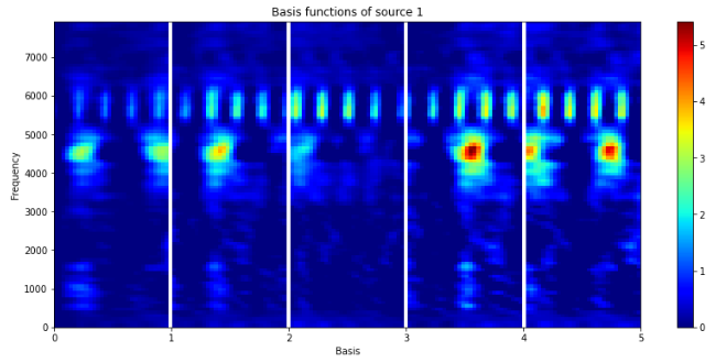
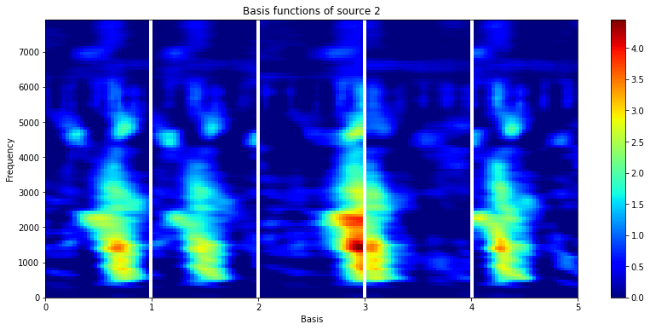
After preparing the training spectrogram, we can train a model with source_separation. NMF learns a set of basis functions to reconstruct the training spectrogram. In soundscape_IR, we can apply PC-NMF to separate the basis functions into two groups according to their source-specific periodicity. In this example, one group of basis funcitons is associated with deer call (mainly < 4 kHz) and another group is associated with noise (mainly > 3.5 kHz). Save the model for further applications.
from soundscape_IR.soundscape_viewer import source_separation

# Define model parameters
model=source_separation(feature_length=30, basis_num=10)

# Feature learning
model.learn_feature(input_data=sound_train.data, f=sound_train.f, method='PCNMF')

# Plot the basis functions of two sound source
model.plot_nmf(plot_type='W', source=1)
model.plot_nmf(plot_type='W', source=2)

# Save the model
model.save_model(filename='./data/model/deer_model.mat')
Deployment and spectrogram reconstruction
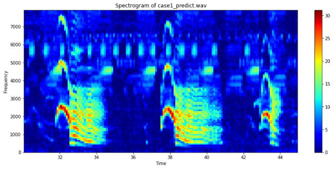
Generate another spectrogram for testing the source separation model.
# Prepare a spectrogram
sound_predict=audio_visualization(filename='case1_predict.wav', path='./data/wav/', offset_read=30, duration_read=15,
                                    FFT_size=512, time_resolution=0.1, prewhiten_percent=10, f_range=[0,8000])
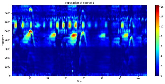
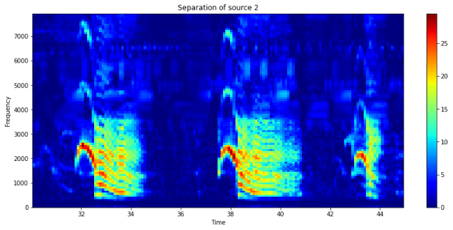
Load the saved model and perform source separation. After the prediction procedure, plot the reconstructed spectrograms to evaluate the separation of deer calls and noise.
# Deploy the model
model=source_separation()
model.load_model(filename='./data/model/deer_model.mat')
model.prediction(input_data=sound_predict.data, f=sound_predict.f)

# View individual reconstructed spectrogram
model.plot_nmf(plot_type = 'separation', source = 1)
model.plot_nmf(plot_type = 'separation', source = 2)
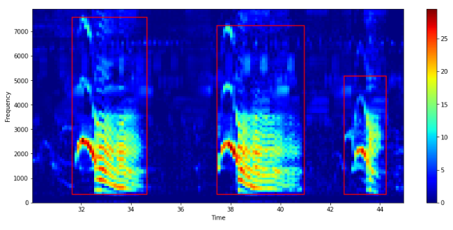
Run spectrogram detection
With the reconstructed spectrogram, we can use the function spectrogram_detection to detect the presence of target signals (e.g., deer calls). This function will generate a txt file contains the beginning time, ending time, minimum frequency, and maximum frequency of each detected call. Explore the detection result in Raven software.
from soundscape_IR.soundscape_viewer import spectrogram_detection

# Choose the source for signal detection
source_num=2

# Define the detection parameters
sp=spectrogram_detection(model.separation[source_num-1], model.f, threshold=5.5, smooth=1, minimum_interval=0.5,
                           filename='deer_detection.txt', path='./data/txt/')