Run batch analysis

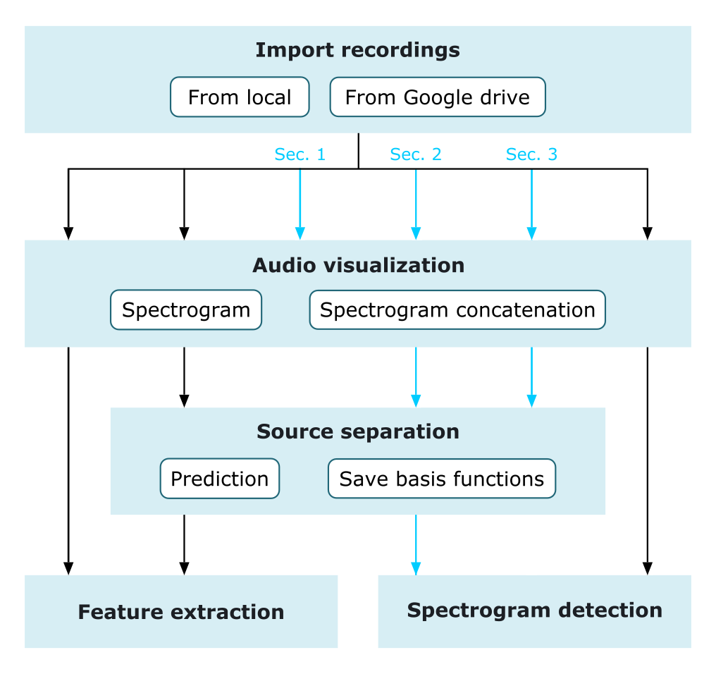
This tutorial introduces the application of the module batch_processing in analyzing a large amount of audio recordings. This tutorial contains three sections:

Generating a concatenated spectrogram from multiple recordings
Applying model-based source separation to detect target sounds
Performing adaptive and semi-supervised source separation to assess acoustic diversity

Spectrogram concatenation

In order to build a robust source separation model, we often need to use a large amount of annotated sounds for model training. The module batch_processing allows to extract annotated clips from multiple recordings and subsequently generates a concatenated spectrogram.

At first, create a folder and copy a set of annotated recordings to the folder. Enter the folder path in folder and the extended file name of the associated txt files containing annotations (generated by using Raven software) in annotation_extension. For example, if our recording files are named using the structure of Location_Date_Time.wav and txt files are Location_Date_Time.Table.1.selections.txt, please enter annotation_extension='.Table.1.selections.txt'.

Then, define spectrogram parameters and set folder_combine=True in batch_processing.params_spectrogram. By doing this, batch_processing will combine all the recordings from the folder and generate a concatenated spectrogram according to the associated annotations. If only a portion of recordings in the folder is needed, we can specify the beginning file number (start from 1) in start and the number of recordings in num_file.

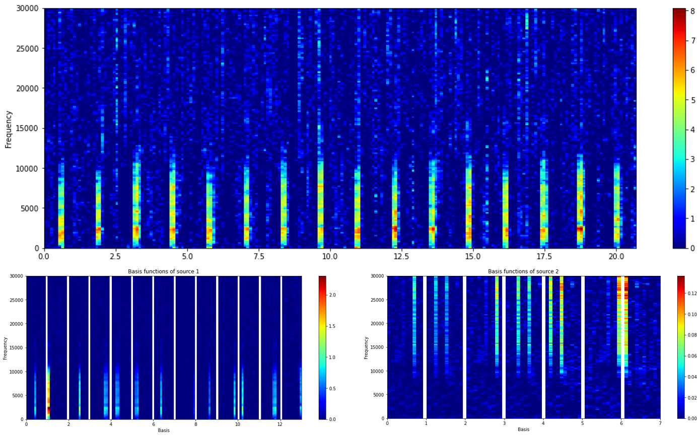
After performing batch_processing, a concatenated spectrogram is saved in batch_processing.spectrogram, and we can plot the concatenated spectrogram by using matrix_operation().plot_lts.

from soundscape_IR.soundscape_viewer import batch_processing
from soundscape_IR.soundscape_viewer import matrix_operation
from soundscape_IR.soundscape_viewer import source_separation

# Assign the folder path contains annotated recordings
path='./data/batch/sec1_2/'

# Define parameters
batch = batch_processing(folder=path, file_extension='.wav', annotation_extension='.Table.1.selections.txt')
batch.params_spectrogram(FFT_size=1024, f_range = [0,30000], environment='wat', prewhiten_percent=20, time_resolution=0.05, padding=0.5, folder_combine=True)
batch.run(start=1, num_file=2)

# Plot concatenated spectrogram
matrix_operation().plot_lts(batch.spectrogram, batch.f, fig_width=18, fig_height=6, lts=False)

# Train a source separation model using PC-NMF
model=source_separation(feature_length=10, basis_num=20)
model.learn_feature(input_data=batch.spectrogram, f=batch.f, method='PCNMF')

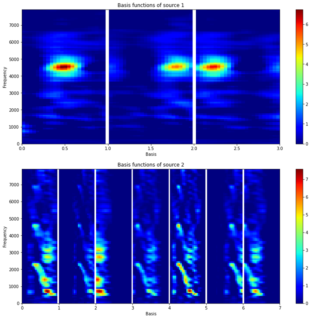
# Plot the basis functions of each source
model.plot_nmf(plot_type='W', source=1)
model.plot_nmf(plot_type='W', source=2)

Source separation and spectrogram detection

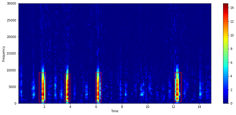
This section demonstrates the use of a source separation model in batch_processing to detect target sounds from a set of unannotated recordings.

Here, we set folder_combine=False to sequentially process recordings. In addition, we add batch_processing.params_separation and batch_processing.params_spectrogram_detection to import the model and to run an energy detector. In batch_processing.params_spectrogram_detection, we can specify multiple sources (e.g., source=[1,2]) to separately detect regions of interests from different sources.

Detection results will be saved as txt files (with source number after the original filename), using the same annotation format prepared via Raven software. The plotting function of detection results can be deactivated by setting show_result=False.

from soundscape_IR.soundscape_viewer import batch_processing

# Assign the folder path of unannotated recordings and the path for saving detection results (in txt format)
path='./data/batch/sec1_2/'
save_path = './data/txt'

# Define parameters
batch = batch_processing(folder=path, file_extension='.wav')
batch.params_spectrogram(FFT_size=1024, environment='wat', prewhiten_percent=20, time_resolution=0.05, f_range=[0, 30000])
batch.params_separation(model)
batch.params_spectrogram_detection(source=1, threshold=6, smooth=1, pad_size=0, path=save_path, minimum_interval=0.5, show_result=True)
batch.run(start=3, num_file=2)

Adaptive and semi-supervised source separation

The application of source separation in batch_processing also enables the use of adpated and semi-supervised learning methods in extracting acoustic features associated with target sounds displaying varied features and unknown sounds.

At first, load a source separation model previously trained. Then, define adaptive_alpha and additional_basis in batch_processing.params_separation to enable adpated and semi-supervised source separation. Note that we can assign multiple values in adaptive_alpha for different sound sources. In this example, we allow basis functions associated with deer calls to adapt from the variations among different calling individuals.

In batch_processing.params_separation, set save_basis=True to save the basis fuctions learned in source separation procedures into a mat file.

from soundscape_IR.soundscape_viewer import source_separation
from soundscape_IR.soundscape_viewer import batch_processing

# Load a source separation model
model=source_separation()
model.load_model('./data/model/KT08_linear_fl24_bn10.mat')

# Assign the folder_id of unannotated recordings and the path for saving basis functions (in mat format)
path='./data/batch/sec3/'
save_path='./data/mat'

# Define parameters
batch = batch_processing(folder=path, file_extension='.wav')
batch.params_spectrogram(FFT_size=512, time_resolution=0.1, window_overlap=0.5, prewhiten_percent=25, f_range=[0,8000])
batch.params_separation(model, adaptive_alpha=[0,0.2], additional_basis = 0, save_basis=True, path=save_path)
batch.run()

# Load the basis functions from a specific mat file
load_basis=source_separation()
load_basis.load_model('./data/mat/KT08_20171118_123000.mat', model_check=False)

# Plot the basis functions of each source
for i in range(load_basis.source_num):
  load_basis.plot_nmf(plot_type = 'W', source = i+1)

Aftering performing adapted or semi-supervised source separation, we can use batch_processing to load all basis functions for visualizing acoustic diversity.

Here, we use batch_processing.params_load_result to load a large number of mat files. Please enter the filename information of the mat files so that batch_processing can extract the recording date and time from each mat file. For example, if the file name is ‘KT08_20171118_123000.mat’, please enter initial='KT08_' and dateformat='yyyymmdd_HHMMSS'. After the loading procedure, a source separation model contains all the basis functions is saved in batch_processing.model, and we can use model.plot_nmf() to plot basis functions or extract basis functions from model.W and model.W_cluster.

from soundscape_IR.soundscape_viewer import batch_processing

# Assign the folder path of saved mat files
mat_path='./data/mat'

# Define parameters
batch = batch_processing(folder=mat_path, file_extension='.mat')
batch.params_load_result(data_type='basis', initial='KT08_', dateformat='yyyymmdd_HHMMSS')
batch.run()

# Plot the entire set of basis functions
idx = batch.model.W_cluster == 1
batch.model.W = batch.model.W[:,idx][:,::7]
batch.model.plot_nmf(plot_type='W')

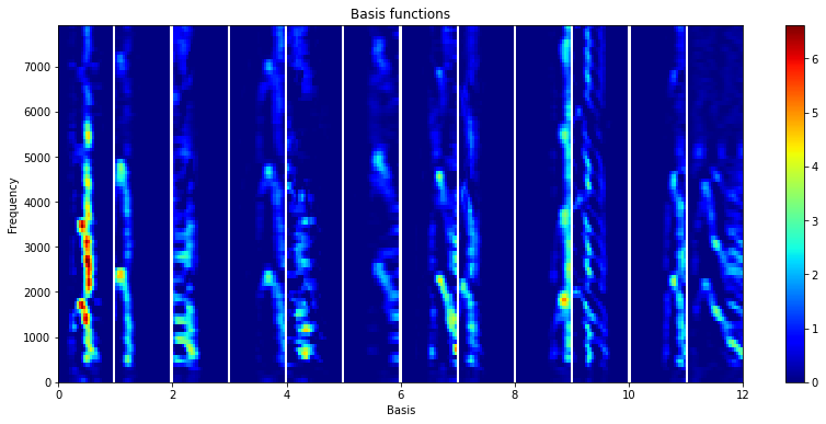
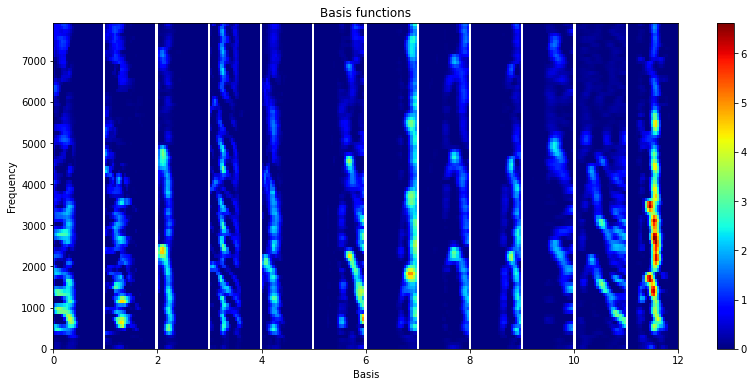
With adapted source separation, we can obtain a set of basis functions associated with different sound types. We choose one feature from the adapted basis functions in each mat file and project these basis functions on an one-dimensional axis using Uniform Manifold Approximation and Projection (UMAP). The UMAP coordinate summarizes the spectral variations of the adapted basis functions. By sorting the adapted basis functions according to their UMAP scores, the basis functions at the left part are mostly characterized by burst-pulses, and the basis functions at the right part are tonal sounds with a few harmonics.

import umap
import numpy as np

# Performing UMAP analysis on the adapted basis functions
model = umap.UMAP(n_neighbors=3, n_components = 1)
data_umap = model.fit_transform(batch.model.W.T)

# Display the spectral variations of the adapted basis functions
idx = np.argsort(data_umap[:,0])
batch.model.W = batch.model.W[:,idx]
batch.model.plot_nmf(plot_type='W')